Training
Note: Segmentation using Deep Learning requires the Deep Learning extension to the 2D Automated Analysis module. The Image-Pro Neural Engine must be installed. Installing the Image-Pro Neural Engine
Train deep learning models using the AI Deep Learning Trainer.
Click on the AI drop-down menu in the Segment tool group on the Count/Size tab, select Deep Learning Trainer. The AI Deep Learning Trainer panel opens.
Default Image-Pro AI models are System Locked and can not modified with further training. If you wish to modify one of these models with additional training, clone it first. The cloned model is fully trainable.
Cloning, Editing and Adding Deep Learning Models
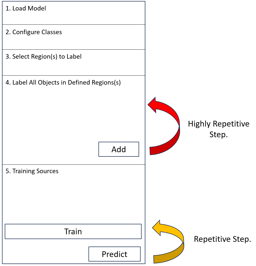
The Deep Learning Trainer is divided into five sections
-
Load Model
-
Click the Load button, select the model that you wish to train, and click Open.
-
-
Configure Classes
-
Click on the Color Picker to configure the appearance of training objects.
-
Show or Hide classes of training objects by clicking on the Eye control.
-
Edit class names by clicking on the name field.
-
-
Select Region(s) to Label
If you wish to label all of the objects in the whole image, skip this step. If you only wish to label the objects in a specific region, or specific regions of the image ensure that these regions are enclosed within regions of interest using the tools in this section.
Note: Failure to label objects of interest that are not excluded from regions of interest is likely to degrade your model.
-
Label All Objects in Defined Region(s)
-
Select your labeling method and add labels to the active image. You can choose between:
 Draw Manually
This labeling method is recommended when you are training a class of objects for which existing segmentation methods and deep learning models do not return any useful results.
Useful drawing and editing tools can be selected directly from the Label All Objects in Defined Region(s) section of the trainer.
When you finish adding and editing labels for your objects of interest, ensure that the correct Training Channel and Seed Channel (if applicable) are selected and click Add.
You can then either open another image and add more labels, or move to Step 5 of the Deep Learning Trainer.
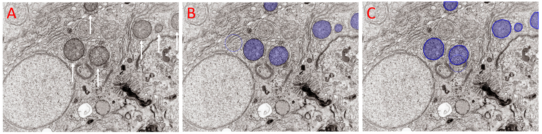
Figure illustrating addition of labels to objects of interest with Draw Manually selected in the Deep Learning Trainer. A) Field of View with several objects of interest arrowed. These objects can not be segmented with Smart or Threshold segmentation. B) The same field of view with the objects of interest drawn with the Brush tool before validation. C) The same field of view with the brushed objects validated. The validated objects can be added to the model's training data by clicking the Add button. Image: Kevin Mackenzie, University of Aberdeen License: Attribution 4.0 International (CC BY 4.0)
Segmentation
This labeling method can be used if you are able to generate useful segmentation from either Smart Segmentation or Threshold Segmentation.
Clicking on the Smart Segmentation or Threshold Segmentation button in the Label All Objects in Defined Region(s) section of the Deep Learning trainer will open the appropriate segmentation panel. Use the segmentation panel to find and count objects in your image.
You can then select the Draw Manually option to delete, edit and add labels. When you are happy with the labels ensure that the correct Training Channel and Seed Channel (if applicable) are selected and click Add.
You can then either open another image and add more labels, or move to Step 5 of the Deep Learning Trainer.
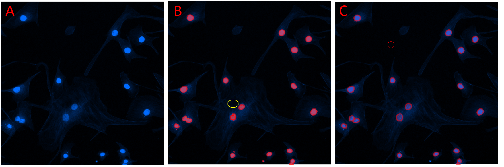
Figure illustrating addition of labels to objects of interest with Segmentation selected in the Deep Learning Trainer. A) Field of view showing several objects of interest. B) The same field of view after the Smart Segmentation button was selected in the Deep Learning Trainer. A smart segmentation recipe was added (reference objects are shown) and the objects were counted. C) The same field of view after the counted objects were manually edited. The objects can be added to the model's training data by clicking the Add button.
Predict with Existing
This labeling method can be used when a model is available that is partially trained, but requires improvement with the addition of additional training objects. Indeed, you may use the model that you are in the process of training to find objects, then manually edit these objects.
This approach is suggested by Pachitariu and Stringer(2022), who stated "Another class of interactive approaches known as ‘human-in-the-loop’ start with a small amount of user-segmented data to train an initial, imperfect model. The imperfect model is applied to other images, and the results are corrected by the user".
Clicking on the Prediction button in the Label All Objects in Defined Region(s) section of the Deep Learning trainer will open the Deep Learning Prediction panel. Use the Deep Learning Prediction panel to predict objects in your image.
You can then select the Draw Manually option to delete, edit and add labels. When you are happy with the labels ensure that the correct Training Channel and Seed Channel (if applicable) are selected and click Add.
You can then either open another image and add more labels, or move to Step 5 of the Deep Learning Trainer.
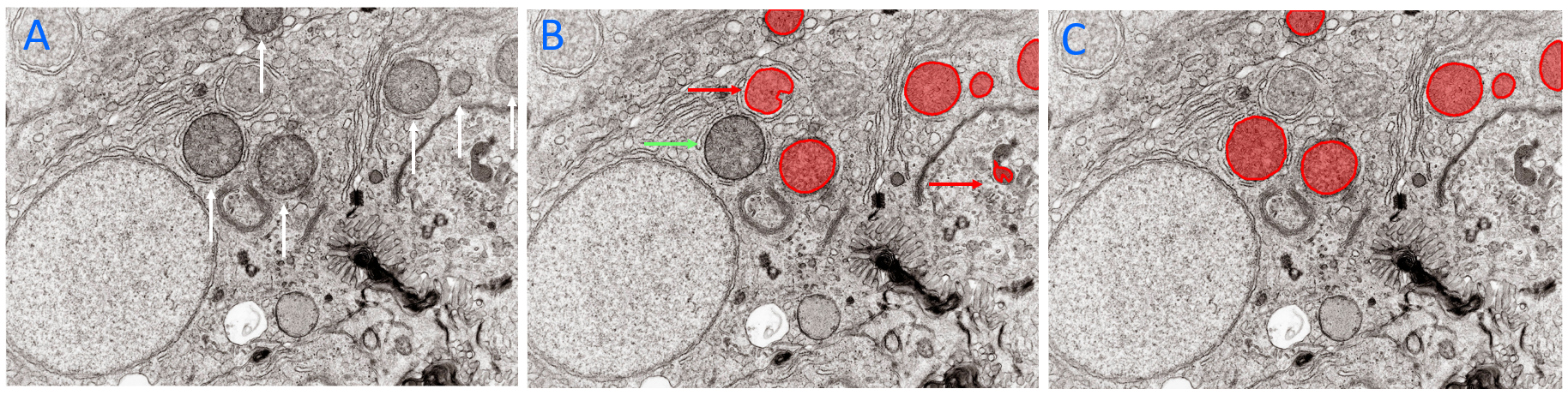
Figure illustrating addition of labels to objects of interest with Predict with Existing Model selected in the Deep Learning Trainer. A) Field of View with several objects of interest arrowed. B) The same field of view after the Predict with Existing Model button was selected in the Deep Learning Trainer. A deep learning model was used to predict the objects of interest in the image. Note the presence of two false positives (red arrows) and false negative (green arrow). C) The same field of view after the counted objects were manually edited. The objects can be added to the model's training data by clicking the Add button. Image: Kevin Mackenzie, University of Aberdeen. License: Attribution 4.0 International (CC BY 4.0)
Note: Ensure that all of the instances of your objects of interest are labeled. Unlabeled instances will be considered as background by the model, generating a less effective model. If you don't want to add labels to the whole image, add a Region of Interest to the Image (step 3) and add labels to all of the instances of the object within the Region of Interest.
-
-
Training Sources
The number of labels that you have added to the active image is displayed under Current Labels to the left of the Add button.
The number of images, labels, and the mean diameter (Ø) of labels that you have previously added to your training data is displayed under Training Set to the right of the Add button.
A time stamp shows the last time that labels were added to the training data.
When all of the objects of interest in your image, or within your region of interest have been labeled correctly, click the Add button.
In the dialog that opens ensure that the Source Image, Training Channel and optional Seed Channel (if supported by your model's architecture) are correct, then click Add.
Note: If you have already added labels to the Training Set from the active image, the dialog will show an options to Replace All or Append.
Click Replace All if you have corrected labels in a region that was previously labeled.
Click Append if you have added new labels within a new region of interest.
Each time you click Add the number of images in the Training Set is incremented by 1, the number of labels in the Training Set is incremented by the number of labels on the active image, mean diameter (Ø) of the labels is re-calculated and the time stamp updates.
Train
As soon a labels are added to the Training Set, the Train button is activated. You can train as often as you wish after adding labels.
-
From the Train drop-down menu, configure the Use Training Graph selection. Selecting this option is recommended for training, the training graph provides useful feedback on the effectiveness of training.
-
Click Train.
-
The Train dialog is displayed.
-
Configure the Number of Steps (if supported by your model's architecture).
-
Configure the number of Epochs.
-
Configure the Train Size Model check box (if supported by your model's architecture). When selected, a second deep learning model dedicated to predicting the size of your objects of interest (in the prediction panel) is trained when the training of the main model completes.
-
Click Start to initiate training.
-
-
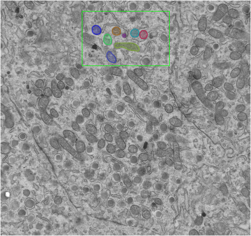
Figure illustrating the partial labeling of an image for Deep Learning Training. A region of interest has been added to the image, all objects of interest within the Region of Interest have been labeled.
Note: An Epoch is a phase in the training process that contains multiple iterations or Steps. After each Epoch the model is tested, if the Loss function is reduced, the model is saved. The number of Steps is calculated automatically based on the training data-set size by CellPose models, and is determined by the user for StarDist and BaseUNET models.
You can monitor the progress of training in the Deep Learning Output panel and graphically in the Training Graph panel. The Loss Function is calculated after each training epoch. The Loss function is measurement of the difference between the training objects and predicted objects. The lower the loss function, the more accurate the model.

Text output from the Deep Learning Output panel for a single training epoch of a Cellpose model. Note Values for Loss and LR (Learning Rate)
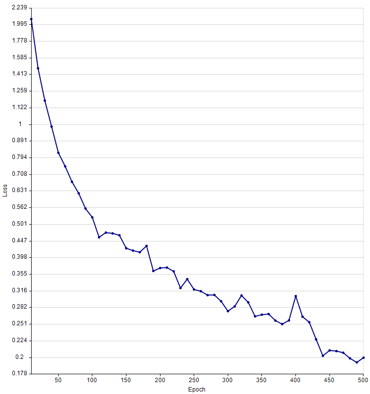
The Training Graph for a Cellpose model, trained from scratch. The model was based on 12 images and 518 labels. The loss function was reduced from 2.07 to 0.199 over 500 epochs.
After training, click Predict to load the newly trained model into the Predication panel. You can run tests to determine if your model is sufficiently trained, or whether you need to add additional training data and re-train.
Adding additional training objects
Additional training objects can be added to a trained model and training can be repeated. New training data is appended to existing training data in the training graph.
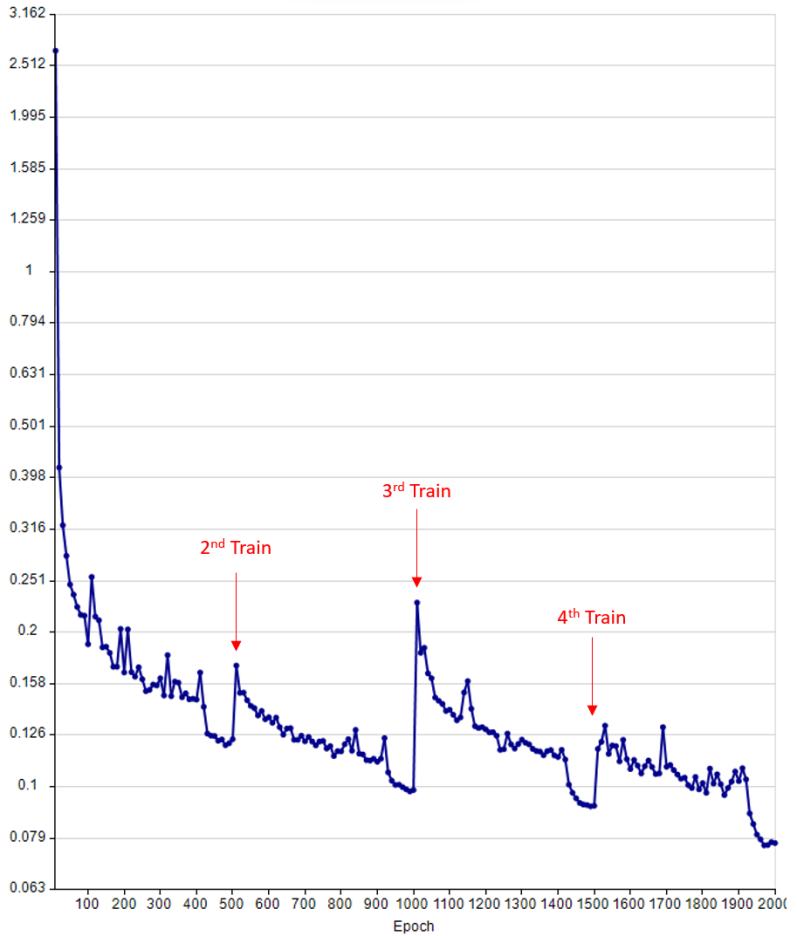
The training graph of a Cellpose model after four rounds of training. Additional training data was added before each round of training. Each round consisted of 500 epochs. The start of the 2nd, 3rd, and 4th rounds of training are arrowed. Note: The loss function frequently increases for the initial epochs after adding new training data.
Note: Sections 4 and 5 can be applied iteratively. Labels can be added from multiple images, and models can be re-trained whenever new training sources have been added.
Restore Points
Each time you train a model, a restore point is made (with default settings). A restore point represents a record of the model at the point that the Train button was clicked. Models can be reverted to any restore point, removing the effect of any training made after the restore point was added.
Restore points make all new training undo-able, giving you the freedom to add experimental or low quality data to your model safe in the knowledge that it can be removed later should the model not benefit from the change.
To see the restore points associate with a model, click on the History button from the Training Sources section of the Deep Learning Trainer. The Model History dialog will open.
The Model History dialog displays two tables which help you to keep track of your model's origins and training sources.
Training History Table
Each row of this table shows data for each restore point (RP) :
| Date/Time | Images | Labels | Epochs | Loss | Restore | Delete |
|---|---|---|---|---|---|---|
| The time of RP creation | The number of training images. | The number of training labels. | Number of training epochs applied. | The Loss function for the RP | Click this button to revert the model to this RP. | Click this button to remove the RP from the history. |
Restore: Click this button (which is located in the table) to revert the model to its state when the restore point was created. The current state of the model is automatically added to the history as a new restore point.
Delete: Click this button (which is located in the table) to delete a restore point.
Reset Model: This option resets the model to a fully untrained state. A restore point of the current state is automatically added if this options is selected.
Create: This option adds a restore point of the model's current state.
Auto-Create Restore Points: With option selected, restore points are added to the history every time the Train button is clicked. With this option deselected, you can manually add restore points by clicking Create.
Model Ancestors
This table is only populated if a model was generated by cloning a model.
Each row represents a generation of a cloned model's ancestors, with the top row representing the parent model (from which the current model was cloned), the next row representing the grandparent model (from which the parent model was cloned) etc.
| Name | Date/Time | Images | Labels | Epochs | Loss |
|---|---|---|---|---|---|
| The name of the ancestor model | The time stamp of the ancestor model cloning. | The number of images used to train the ancestor. | The number of labels used to train the ancestor. | The number of epochs over which the ancestor was trained. | The Loss function of the ancestor model. |
Reviewing and Editing Training Data
The images that have been used to train a model can be reviewed by clicking on the Show Sources button in the Model History dialog. Training images are displayed in the file browser. Double click on an image's thumbnail in the browser to open it in the Image-Pro workspace where the labels that were added during training can be reviewed.
If you wish to remove an image from the training data, right click on the image's thumbnails in the file browser and select Delete. Future rounds of training will not include the deleted image.
Adding Example Images
After satisfactory testing of a newly trained model, you can click the Add Screenshot button in the AI Deep Learning Prediction panel to save the active image with all of the predicted objects as an 'Example' image that can be viewed from The Model Manager.
How many training objects are required to train a deep learning model?
While this is the first question most people are likely to ask before embarking on a deep learning model training project, providing a simple definitive answer is not possible. The number of objects required is dependent of factors such as whether you model is new or cloned (and how different your objects of interest are to those on which the ancestor model was trained), the consistency of appearance and size of your objects of interest, and the consistency of the background.
Valuable insight can be gained from the creators of each architecture.
UNET
The creators of U-NET state that this architecture can be trained with ‘very few’ annotated images (Ronneberger et al. 2015). Our experience of working with this architecture supports this conclusion with effective models being made from as few as 2 or 3 annotated images in some cases.
Cellpose
Pachitariu and Stringer (2022) noted that pre-trained Cellpose models can be fine tuned from as few as 500 to 1000 user annotations. In contrast, they noted that when starting from untrained models as many as 200,000 annotations may be required.
StarDist
The StarDist FAQs state that “We have often seen good results from as few as 5-10 image crops each having 10-20 annotated objects (in 2D)”. They add the important caveat that “your mileage may vary substantially”.
Frequently Asked Questions (FAQ) — StarDist documentation
Given the high degree of uncertainty in the number of annotations required to train a model of any architecture, we recommend that you start training your model with a small number of objects, followed by training and testing of your model. Add more objects and repeat training as often as necessary in order to train a model to the standard that you require.
Bibliography
Ronneberger, O., Fischer, P., Brox T.(2015) U-Net: Convolutional Networks for Biomedical Image Segmentation.
Medical Image Computing and Computer-Assisted Intervention (MICCAI), Springer, LNCS, Vol.9351: 234--241, 2015, available at arXiv:1505.04597 [cs.CV]
Stringer, C., Wang, T., Michaelos, M. & Pachitariu, M. (2021) Cellpose: a generalist algorithm for cellular segmentation. Nat Methods 18, 100–106. https://doi.org/10.1038/s41592-020-01018-x
Learn more about all features in Count/Size